Data Processing
1) By joining the MEPS Medical Conditions file (COND) and the Prescribed Medicines file (RX) via the Condition-Event Link file (CLNK), we created a dataset where each row was a prescription event: one instance of a person filling or refilling a drug, including the name of the drug and for what condition it was prescribed. (281,158 rows, 11 variables.)
2) After removing refills (so each patient–drug–condition combination was counted only once), removing rare conditions and drugs (<25 occurrences), and aggregating the drugs into 16 therapeutic classes, we created a condition–drug co-occurrence matrix: each of the 206 rows was a condition, each of the 16 columns was a drug class, and each cell held the number of times they occurred together in a prescription event. This matrix answers the question, “How many people in the sample were ever prescribed a drug in class D for condition C?”
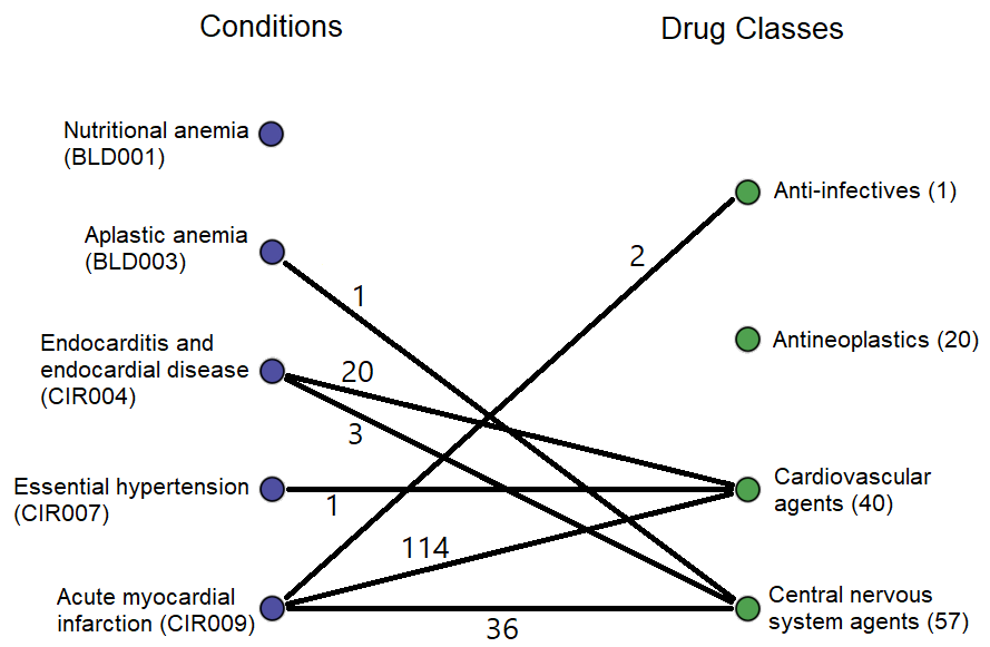
Conceptually, this matrix represents a bipartite graph connecting conditions to the classes of drugs prescribed for them, with edge weights equaling the number of people to whom such a prescription was given. That graph would look like this, but with 201 more conditions and 12 more drug classes (the weights are from the real data).
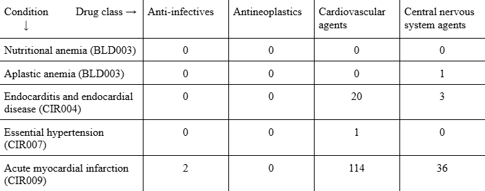
Literally, the matrix looks like this (with 12 more columns and 201 more rows).
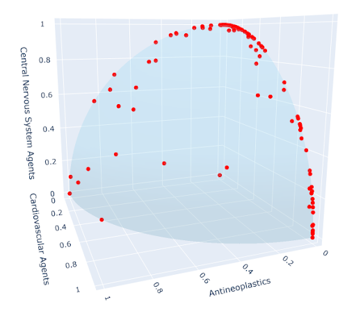
3) Since we were interested only in which drugs were typically prescribed for each condition, not how often the conditions occurred, we performed a final step: normalization. After normalization, each vector has an L2 norm of 1, so the data can be visualized as points on the unit sphere in 16 dimensions, all lying in the positive orthant or on an axis bordering it. Using only the first three dimensions, we get the figure at left; try to envision the impossible, an analogous figure in 16 dimensions, and you’ll have a good understanding of the final data structure.
The higher the value of a coordinate, the more often drugs of that class are prescribed for that condition.
Clustering
We used three clustering methods:
- K-means
- Hiearchical agglomerative clustering (HAC)
- Mixture of von Mises–Fisher distributions (vMF) (I was responsible for this model, which I borrowed from Banerjee, Arindam; Dhillon, Inderjit S.; Ghosh, Joydeep; Sra, Suvrit (2005). Clustering on the Unit Hypersphere using von Mises-Fisher Distributions. Journal of Machine Learning Research, 6, 1345–1382.)
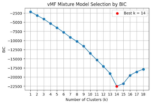
Using BIC, the optimal number of clusters was 14 (click to show plot).
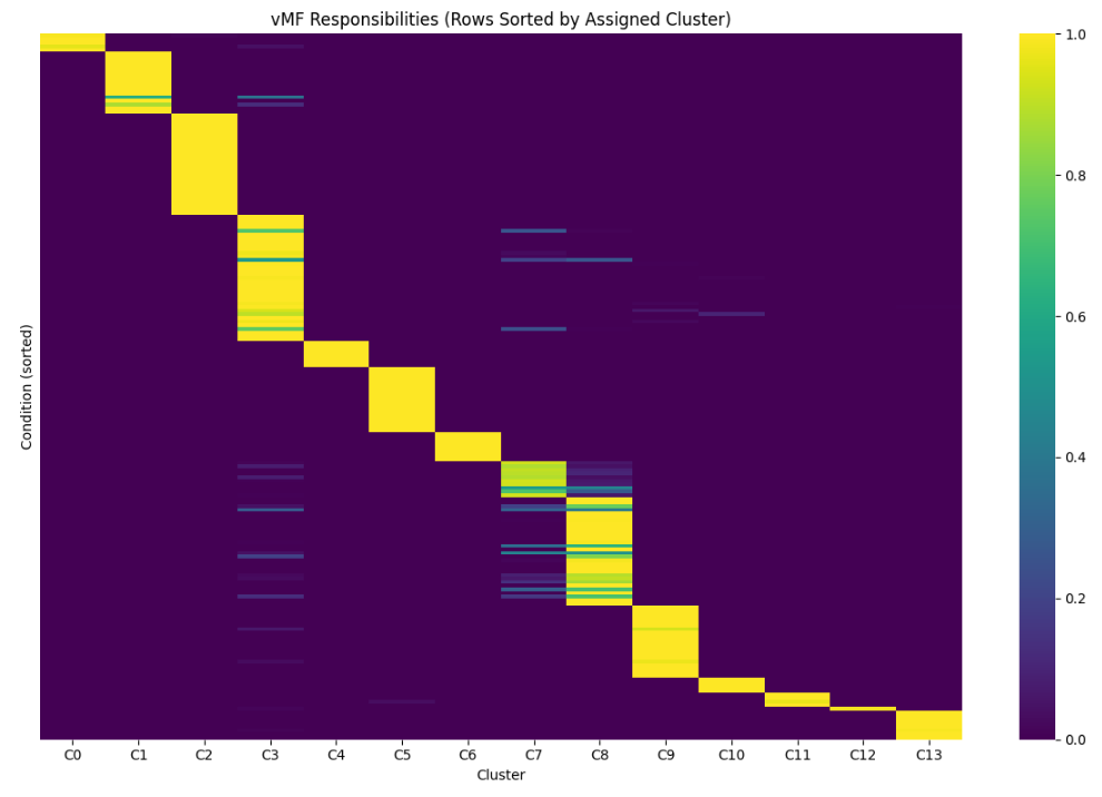
The soft cluster assignments were mostly confident, but there is some uncertainty about the boundaries between a few of the clusters, most notably 3, 7, and 8 (click to show plot; the lighter the color, the higher likelihood the point represented by the row belongs to the cluster represented by the column).
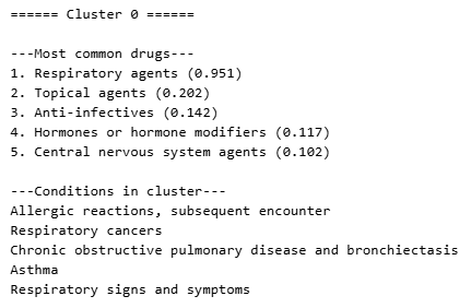
At right (or below, on mobile) is an example cluster. For each cluster, we found the mean vector—the “characteristic condition” of that cluster—and used it to identify the cluster’s typical prescription pattern. The number in parentheses is the coordinate, representing how frequently the drug class is prescribed for conditions in the cluster. (Keep in mind the coordinates don’t have a meaningful unit; the most specific valid interpretation is “higher means more frequent.”)
All three methods produced similar clusters with similar themes. We identified cluster themes manually by looking at the types of conditions in them and the types of drugs most germane to it, then we had an LLM do the same exercise to verify our conclusions. These, roughly, were the cluster themes (the numbers are arbitrary, just identifiers):
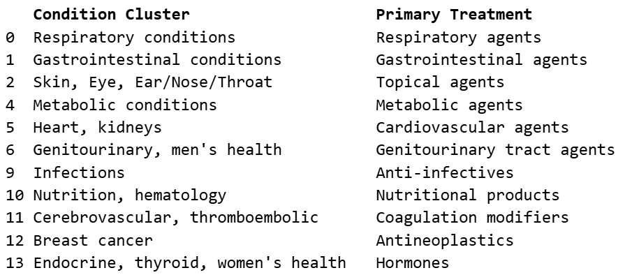
Click here to see the complete set of clusters.
Takeaways
Most of the analysis validates common-sense conclusions. Of course most respiratory conditions are treated similarly, predominantly with respiratory agents; of course most gastrointestinal conditions are treated similarly, predominantly with gastrointestinal agents; etc. Where clusters are clean, no questions are raised.
Three of the clusters are less clear. To me, these are the interesting ones. I’ll conclude with a few potential questions:
The division between cluster 7, which we’ve informally labeled as “central nervous system (CNS) disorders,” and cluster 8, which we’ve called “mental health conditions,” is blurry. (In fact, k-means and HAC didn’t even make them distinct clusters.) Cluster 7 is treated almost exclusively by CNS agents, while cluster 8 is treated primarily by CNS agents but also has a very common secondary drug class: psychotherapeutic agents. Why are these clusters so intertwined? It would be satisfying if, waiting to be unearthed here, there were two clusters with different primary drug classes: one for conditions best treated by CNS agents, and one for conditions best treated by psychotherapeutic agents. Can further study of these conditions reduce the variation in how cluster 8 is treated, leading to the emergence of two distinct groups?
Cluster 3 is the largest, has the largest variety in prescriptions, and has many low-confidence assignments. K-means and HAC both produced a similar cluster. This cluster is a sort of mixed bag: no strong unifying type of condition, no strong unifying treatment. Every condition in this cluster, then, raises questions of its own. If there isn’t a consistently applied treatment method, it implies a strong, effective treatment method isn’t known (or else it would be used consistently); can one be discovered? Or, if a condition in this cluster does have a consistent treatment, then it’s categorized here because there are few or no similar conditions, begging the question “what makes that condition so unusual?”